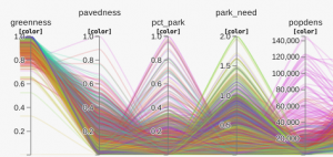
 I stumbled across the City Nature project at Stanford via some interesting interactive data visualization they have created like the comparison between natural and social variables and the Naturehoods Explorer for 34 US cities.
One of the comments in the comparison chart (first project link), was lack of clear relationships between any of the provided variables. As I’m a glutton for punishment, I thought I’d give it a go.
With the addition of only two variables at the City level to the data provided by the Naturehoods Explorer, I was able to get a good start on a linear regression model. The two variables added are city population and number of parks in the city.
Below are results to linear regression models through R.
> summary(lm(park_count ~ . , data =g2))

Call:
lm(formula = park_count ~ ., data = g2)

Residuals:
    Min      1Q  Median      3Q     Max
-267.25  -42.72   -2.30   56.81  189.01

Coefficients:
              Estimate Std. Error t value Pr(>|t|)
(Intercept)  5.636e+01  4.260e+01   1.323 0.185897
greenness    4.061e+02  3.640e+01  11.157  < 2e-16 ***
pavedness   -1.881e+01  1.861e+01  -1.011 0.312164
pct_park    -7.069e+01  1.416e+01  -4.994 6.30e-07 ***
park_need   -7.382e+00  4.833e+00  -1.528 0.126742
popdens      4.525e-04  1.780e-04   2.542 0.011090 *
h_inc        5.544e-04  1.293e-04   4.288 1.87e-05 ***
home_val    -2.578e-04  2.129e-05 -12.110  < 2e-16 ***
pct_own      4.294e+01  1.184e+01   3.627 0.000292 ***
diversity    5.461e-01  9.816e-02   5.563 2.91e-08 ***
nonwhite    -8.912e+01  7.936e+00 -11.230  < 2e-16 ***
parkspeak   -2.449e+02  3.087e+01  -7.933 3.12e-15 ***
lng         -6.429e-02  1.508e-01  -0.426 0.669870
lat         -7.898e+00  3.937e-01 -20.060  < 2e-16 ***
population   1.649e-05  1.372e-06  12.023  < 2e-16 ***
---
Signif. codes:  0 ‘***’ 0.001 ‘**’ 0.01 ‘*’ 0.05 ‘.’ 0.1 ‘ ’ 1

Residual standard error: 77.24 on 2646 degrees of freedom
Multiple R-squared: 0.447,	Adjusted R-squared: 0.4441
F-statistic: 152.8 on 14 and 2646 DF,  p-value: < 2.2e-16
I also normalized the fields, except park_count, to get a feel of the relative impact of the individual variables across their very different scales. The estimate indicates a change by one standard deviation of the variable.
> summary(lm(park_count ~ . , data =g3))

Call:
lm(formula = park_count ~ ., data = g3)

Residuals:
    Min      1Q  Median      3Q     Max
-267.25  -42.72   -2.30   56.81  189.01

Coefficients:
            Estimate Std. Error t value Pr(>|t|)
(Intercept) 152.7865     1.4973 102.043  < 2e-16 ***
greenness    21.2528     1.9048  11.157  < 2e-16 ***
pavedness    -2.1510     2.1278  -1.011 0.312164
pct_park     -8.3974     1.6815  -4.994 6.30e-07 ***
park_need    -2.8265     1.8503  -1.528 0.126742
popdens       6.0435     2.3778   2.542 0.011090 *
h_inc        15.4520     3.6039   4.288 1.87e-05 ***
home_val    -43.8665     3.6222 -12.110  < 2e-16 ***
pct_own       8.2300     2.2691   3.627 0.000292 ***
diversity    11.1726     2.0082   5.563 2.91e-08 ***
nonwhite    -21.6853     1.9311 -11.230  < 2e-16 ***
parkspeak   -14.3325     1.8066  -7.933 3.12e-15 ***
lng          -0.9985     2.3418  -0.426 0.669870
lat         -40.1728     2.0026 -20.060  < 2e-16 ***
population   28.5058     2.3710  12.023  < 2e-16 ***
---
Signif. codes:  0 ‘***’ 0.001 ‘**’ 0.01 ‘*’ 0.05 ‘.’ 0.1 ‘ ’ 1

Residual standard error: 77.24 on 2646 degrees of freedom
Multiple R-squared: 0.447,	Adjusted R-squared: 0.4441
F-statistic: 152.8 on 14 and 2646 DF,  p-value: < 2.2e-16
For explanations of the data, collection method, etc., please see the City Nature Project.